Lifecycle Cost of Low-Temperature Units: The Three Accounts Beyond Initial Investment

The conclusion in one sentence

Price comparison in the procurement of low-temperature units usually compares initial investment only, yet the share of initial investment in total cost depends on the operating pattern of the application and is not stable. What really separates the options are the other three accounts: running energy, maintenance and spare parts, and failure downtime loss. They share three characteristics — they occur across years, they depend on the specific operating conditions, and they are invisible at the comparison stage. This article therefore gives no cost figures; it gives a calculation method for each of the three accounts and the steps for converting them to a common basis. The core judgement is this: in continuously operating production applications the three later accounts usually carry more weight than initial investment; in intermittently used laboratory applications the cost of downtime time can exceed the cost of energy. The three cost items have different weight structures and cannot be handled with a single comparison template.

Scope of discussion

• This article discusses the cost composition and calculation methods for -60℃ evaporating temperature class low-temperature units; it does not discuss specific models, quotations or brands.
• All performance figures (cooling capacity, input power, COP, pull-down time and so on) and business parameters (electricity tariff, annual running hours, downtime loss and so on) are given throughout as placeholders (of the form {{制冷量}}) and must be filled in from measurement, the accompanying technical documentation, or the user's own business data.
• No data of the kind of price, energy consumption, failure rate or service life is given; only calculation methods and an information checklist.
• The cost basis is the user's own business; no industry averages or empirical coefficients are provided.
• The reference platform is a -60℃ evaporating temperature class single-stage auto-cascade (SACR) low-temperature refrigeration unit, capacity range 1 – 50 kW (planned family range, not measured values of any single model).
• Cycle and component mechanism are not developed here; see Single-Stage Auto-Cascade (SACR) Cycle Overview.

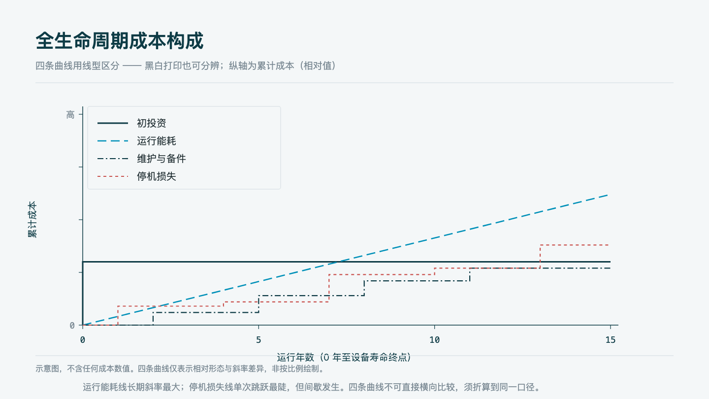
1. The common bias in procurement decisions: initial investment is only one of them

The reason that looking only at initial investment distorts the picture lies not in procurement method but in the comparability of costs. Initial investment occurs once, has an explicit quotation, and can be compared directly; the other three accounts occur spread across years, depend on operating conditions, and require modelling to obtain. With a limited bid-evaluation window, the visible item naturally gains higher weight. This is not an oversight but the inevitable result of a difference in cost visibility.

The cost of a low-temperature unit can be split into four items:

1. Initial investment: the equipment itself, secondary refrigerant and pipework, insulation, electrical and control systems, installation and commissioning.
2. Running energy: electricity consumed, accumulated by actual operating conditions and running hours.
3. Maintenance and spare parts: oil and oil circuit maintenance, drying and moisture control, leak detection, replacement of seals and filter elements, periodic performance testing.
4. Failure downtime loss: downtime duration multiplied by the loss per unit time, plus one-off losses (scrapping of work in progress, re-running of a batch) and the time occupied by warm-up and re-cool-down.

The weight structure of these four items varies sharply with the pattern of use; consider two extremes:

Cost item	Continuously operating production plant	Intermittently used laboratory unit
Initial investment	relatively low weight, amortised once over long running hours	relatively high weight, because annual running hours are few
Running energy	highest weight, proportional to annual running hours {{年运行小时数}}	lower weight, the unit is idle most of the time
Maintenance and spare parts	medium but predictable weight, driven by running hours	weight more affected by maintenance during shutdown and by restarting
Downtime loss	possibly the highest weight, corresponding directly to output and delivery	weight shows up in project schedule and sample value

Basis for the judgement: the annual amount of a cost item equals "amount per occurrence × occurrences per year". Continuous-operation applications push the annual occurrence count high, so energy and downtime loss are amplified; intermittent applications have a low annual occurrence count, initial investment cannot be fully amortised, and its weight rises relatively. The same machine and the same quotation can lead to different reasonable choices in these two kinds of application.

2. The first account: how to calculate running energy

The calculation of running energy proceeds in the following steps: fix the operating point, obtain the input power at that point, and weight by the time distribution.

Step one: make the relationship between cooling capacity and input power explicit. The basic form of energy consumption is input power multiplied by running time. Input power and cooling capacity are linked at a given operating point by the coefficient of performance, that is, at that operating point input power equals cooling capacity divided by the coefficient of performance. The key here is that cooling capacity, input power and coefficient of performance must belong to the same operating point, and that operating point must be fully declared.

Step two: declare the test conditions. A usable performance point must contain at least: evaporating temperature {{蒸发温度}}, condensing temperature {{冷凝温度}}, ambient temperature {{环境温度}}, secondary refrigerant inlet and outlet temperatures {{载冷剂出口温度}}, suction superheat and subcooling ahead of the expansion device. If any one is missing, figures from different sources are not comparable and a conclusion drawn from comparing them does not hold. For the measurement method and the condition-recording requirements see Measuring Cooling Capacity and COP.

Step three: weight by the ambient temperature distribution, not by extrapolating from the design point. Condensing temperature rises with ambient temperature and the pressure ratio rises with it, with the result that cooling capacity falls and input power rises. This means that "design-point energy consumption multiplied by annual running hours" systematically understates annual electricity consumption. A workable approach is to band the year by ambient temperature, take the performance value in each band, and then weight and sum by the hours in that band. The ambient temperature distribution can be obtained from typical meteorological year data for the project location, or recorded on site.

Step four: deal with part load. The rated point is a single condition, while the machine spends most of its running time at part load. Efficiency at part load is strongly related to the modulation method: variable-speed modulation holds efficiency well at part load but is bounded by the compressor's own lower speed limit; hot gas bypass and liquid injection trade cooling capacity for stability and raise the input power per unit of cooling. The calculation must therefore obtain a part-load performance table and confirm the minimum stable load ratio {{最低稳定负荷率}}. For matching on the load side see Pull-Down Rate and Heat Load Matching.

Chaining the four steps above together, the calculation flow for annual running energy cost is:

1. Build the ambient temperature bands and the hours in each band.
2. Build the load distribution (running hours at each load ratio).
3. For each "ambient temperature × load ratio" combination, take the input power {{输入功率}} at that point (if only cooling capacity and coefficient of performance are available, convert from those two).
4. Weight and sum by the combination hours to obtain annual electricity consumption.
5. Multiply by the electricity tariff {{电费单价}} to obtain the annual running energy cost.

Principle when the data is uncertain: if the supplier can provide single-point data only, do not extrapolate from the single point to fill in the other conditions; instead build the calculation framework first using the placeholders {{制冷量}}, {{输入功率}} and {{COP}}, and fill it in after measurement or after the performance table is supplemented. The correctness of the framework matters more than the completeness of the figures, because figures can be filled in later whereas a wrong methodology is carried all the way into the decision.

3. The second account: maintenance and spare parts

The maintenance cost structure of a low-temperature unit differs from that of an ordinary cold store unit. The difference is not that it "costs more" but that there are more items to maintain, degradation is more concealed, and the criteria depend more on trends.

Oil and the oil circuit. Under low-temperature conditions the viscosity of the oil rises and the distribution of oil on heat transfer surfaces and the return path lengthen; at the same time the amount of low-boiling component dissolved in the oil varies with temperature and pressure, which affects the lubricating performance of the oil and its return behaviour. The maintenance action is to test the oil periodically (viscosity, acid value, water content, and system indicators related to oil content) and to change the oil on a schedule {{换油周期}}, rather than waiting until the oil level or oil colour is abnormal. For the related mechanism see Oil Circuit at Low Temperature.

Drying and moisture control. Trace moisture remaining in the system migrates with the refrigerant to the cold side and forms an ice blockage in the expansion device or the low-temperature section of the evaporator, showing up as difficulty in pulling the evaporating temperature down or an abnormal pressure difference across the expansion device. Replacing the filter drier {{干燥过滤器更换周期}} is a routine action, but more important is controlling the points at which moisture enters — the depth of evacuation and the holding criteria; see Evacuation and First Start-Up and Vacuum and Leak Detection.

Leak detection frequency. The molecules of the low-boiling component in a mixed refrigerant are smaller and its tendency to leak is higher. The consequence of a leak is not only a reduced charge but a changed component ratio (composition shift), showing up as lower overhead purity after dephlegmation and an evaporating temperature that will not come down — and this process produces no alarm and no obvious external trace of leakage. Leak detection should therefore be carried out as a periodic action {{检漏周期}}, cross-checked against evacuation hold tests and operating parameter trends; the method is given in Vacuum and Leak Detection.

Ageing of seals. The number of cool-down / warm-up thermal cycles a low-temperature unit experiences has a direct effect on the fatigue of elastomeric seals. An intermittently used application goes through more complete thermal cycles per unit time, so the ageing rhythm of its seals differs from that of a continuously operating application, and the replacement interval has to be estimated by thermal cycle count rather than running hours.

Fouling margin of the dephlegmator and the internal heat exchanger. A rising approach on these two heat exchangers shows up directly as a rising evaporating temperature or insufficient subcooling, and is a leading indicator of performance degradation. The maintenance point is to establish an approach baseline and track the trend, rather than waiting until heat transfer has visibly deteriorated before cleaning. For heat exchanger design points see Internal Heat Exchanger and Dephlegmator.

Recommendation for organising the maintenance plan: organise it in three layers rather than driving it by failure.

1. Daily inspection layer: gauge pressure, oil level, suction superheat, subcooling ahead of the expansion device, running current, secondary refrigerant inlet and outlet temperatures. Its purpose is recording and trend comparison; no complex criteria are set.
2. Periodic testing layer: oil testing {{换油周期}}, moisture and filter drier replacement {{干燥过滤器更换周期}}, leak detection {{检漏周期}}, sampling of the refrigerant vapour composition. The criterion is "has it departed from baseline".
3. Shutdown-period work layer: maintenance before a long shutdown, inspection of seals and insulation during the shutdown, confirmation of pressure balance and oil level before restart. For the criteria see Fault Tree and Diagnosis Order.

The baseline for the three layers of criteria comes from the first commissioning records, so data archiving during commissioning is the reference frame for all later maintenance judgements; see Evacuation and First Start-Up.

4. The third account: how to quantify failure downtime loss

This is the account most easily understated, because it is decided not by the equipment but by the user's business. Its basic quantitative form is:

Downtime loss = downtime duration {{停机时长}} × loss per unit time of lost production {{单位时间停产损失}} + one-off losses

Three places where the calculation goes wrong easily:

First, downtime duration is not the same as repair duration. From the failure occurring to the target temperature being restored, the complete duration includes: discovery and diagnosis of the fault, spare parts arriving, the repair work, warm-up {{复温时间}} and re-cool-down {{再降温时间}}. Of these, the warm-up and re-cool-down times are set by the thermal inertia of the machine itself and are unrelated to how fast the repair is done, and the pull-down time {{降温时间}} of a low-temperature unit is usually the longest link in the whole chain. Estimating downtime duration from repair hours alone understates it significantly. For the factors affecting the pull-down process see Pull-Down Rate and Heat Load Matching.

Second, the knock-on effects are not confined to the equipment side. A process interruption causes scrapping of upstream work in progress, postponement of downstream scheduling, and a batch that has to be started again. For a continuous process, one interruption can mean committing a complete batch again; for a laboratory application, an interruption means failed samples and a slipped project milestone. This part has to be expressed with business parameters such as {{单次批次价值}}.

Third, the response cost of emergency repair differs from that of routine maintenance. Response time {{紧急维修响应时间}}, expedited work, travel to a remote site and temporary alternatives all constitute additional cost. Response time itself is a negotiable item that can be written into the procurement conditions.

Recommendation for the calculation: take neither the worst case nor the average, but estimate "expected number of downtime events per year × loss per downtime event", and then run a sensitivity analysis on the number of events. The expected number of downtime events per year depends on two factors: the degradation rate of the machine itself (which can be influenced through the level of maintenance) and the speed with which the user responds to performance departure (which can be influenced through monitoring and recording capability). The latter is manageable; see Remote Monitoring and Data Logging.

5. Converting the three accounts to a common basis

The three classes of cost have different natures and adding them directly distorts the result; they must first be converted to the same annual basis. A workable method is the annualised total cost of ownership:

Annualised total cost of ownership = annualised initial investment + annual running energy cost + annual maintenance and spare parts cost + annual expected downtime loss

Where:

• Annualised initial investment = initial investment × capital recovery factor. The capital recovery factor is set by the discount rate {{折现率}} and the equipment service life {{设备寿命年限}}, and is used to spread a one-off outlay over each year so that it is comparable with the annual amounts of the three later items.
• Annual running energy cost = annual electricity consumption obtained by the weighting method of section 2 × electricity tariff {{电费单价}}.
• Annual maintenance and spare parts cost = under the maintenance plan of section 3, convert the amount and interval of each action into an annual amount (where the interval is in years take it directly; where it is in running hours or thermal cycles, first convert it into occurrences per year).
• Annual expected downtime loss = expected number of downtime events per year × loss per downtime event, where the loss per downtime event is calculated by the formula in section 4.

Completing this calculation requires two classes of information; if either is missing, the calculation can only remain a framework.

To be requested from the supplier:

1. A multi-condition performance table or performance curves, covering at least the actual ambient temperature range and the actual load ratio range; a rated point alone is not accepted.
2. The condition declaration for each performance point: evaporating temperature, condensing temperature, ambient temperature, secondary refrigerant inlet and outlet temperatures, superheat and subcooling. A performance point with missing items cannot be used in the calculation.
3. The part-load modulation method and modulation range, together with the minimum stable load ratio {{最低稳定负荷率}}.
4. Electrical parameters: rated current, starting current, control supply requirements, for checking the distribution system and starting inrush.
5. The maintenance manual and spare parts list, including the recommended interval for each maintenance action {{换油周期}}, {{干燥过滤器更换周期}}, {{检漏周期}}, and the replacement labour hours for key components.
6. The replacement interval and cost structure of key components, for converting maintenance cost into an annual amount.
7. Pull-down and warm-up time curves (if available), for checking the time occupied within downtime duration.
8. The alarm and protection list, for assessing how self-diagnosing a fault is and thereby estimating diagnosis duration.
9. The agreed in-warranty and out-of-warranty service response time {{紧急维修响应时间}}, for estimating downtime duration and emergency repair cost.

To be prepared by the user:

1. Annual running hours {{年运行小时数}}, together with the ambient temperature bands and the hours in each band.
2. Load distribution: running hours at each load ratio, which can be compiled from the process side or estimated from the process rhythm.
3. Electricity tariff {{电费单价}}, including any peak/off-peak structure where applicable.
4. Loss per unit time of lost production {{单位时间停产损失}} and value of a single batch {{单次批次价值}}, provided by the business side.
5. Discount rate {{折现率}} and equipment service life {{设备寿命年限}}, for annualising the initial investment.

Once the basis is unified, what is being compared is no longer a quotation but the sum of four annualised amounts. One caveat: the value of this method is not in producing a precise figure but in making three invisible costs explicit. Even where some parameters can only be given as a range, writing them into the calculation table changes the content of the discussion — from "who is cheaper" to "how many hours will it run, what does one downtime event cost, and who does the maintenance".

Conclusions and basis for judgement

1. Establish the operating pattern first, then compare costs. Continuous operation and intermittent use have different cost weight structures, and the same quotation can lead to different reasonable choices in the two. Basis: the annual amount of a cost item equals the amount per occurrence multiplied by occurrences per year, and the operating pattern directly sets the occurrence count.
2. The energy calculation must be based on multi-condition data and time weighting; it must not extrapolate from the design point. Basis: condensing temperature varies with ambient temperature, cooling capacity and input power vary with it, and single-point extrapolation departs systematically.
3. Performance data must come with a complete condition declaration. Basis: cooling capacity, input power and coefficient of performance correspond to each other only at the same operating point, and data with missing condition items is not comparable.
4. The maintenance cost of a low-temperature unit is set by the number of items to maintain and by how concealed degradation is, not by the price of the equipment. Basis: refrigerant composition, oil, moisture, seals and heat exchanger approach all have to be tracked on a cycle, and degradation shows up in performance indicators rather than alarms.
5. Downtime duration must include warm-up and re-cool-down time. Basis: these two periods are set by the thermal inertia of the machine and are unrelated to repair speed, and in intermittently used applications they can account for the major part of the downtime duration.
6. Convert the four classes of cost to an annualised basis, and request from the supplier a multi-condition performance table, maintenance intervals and an agreed response time. Basis: without these classes of information the annualised calculation cannot be completed and comparison falls back to initial investment alone.

---

This article is a market insight and gives only cost calculation methods and an information checklist; it contains no quotation, manufacturer comparison or product recommendation. Performance figures and maintenance intervals for specific models are governed by the accompanying technical documentation and the contractual technical agreement.